GNSS原理及其应用

GNSS三大作用 定位(Positioning),导航(Navigation),授时(Timing) # Orientation: Development of GNSS Technologies GPS for short, also named NAVSTAR GPS. GPS stands for Navigation Satellite Timing And Ranging Global Positioning System

Overview

Establish	Target	Started	Full Operational Capacity(FOC)
The US	Provides real-time, continuous, all-weather positioning, navigation and timing PNT services globally	1973	1995

GPS Policies

SA(Selective Availability) policy
SPS(Standard Positioning Service) policy
PPS(Precise Positioning Service) policy

Composition

Space segment

Kind of oribit levels Geostationary Earth orbit 36000km 24h Graveyard oribit MEO satellites COMPASS, GLONASS, Galileo, GPS, etc. LEO satallites : ISS, Hubble Iridium

GPS constellation and its geometric distribution

nominally consisits of 24 operational satellities(21 + 3).
Deployed in six evenly spaced orbit planes(A to F).
With an inclination of 55 degrees and with four satellites per plane.
Several active sparesatellites for replenishment are usually operational.
Elliptical orbit with an average altitude of about 20200km.

specifically, DBS uses three difference type: GEO/IGSO(inclined geosystemary orbit)/MEO.(this arrangement reflects some development of BDS)

resection

for any single satellite: $$ \begin{cases} P_r^s &= c(T_r - T^s) \\ T_r &= t_r + \delta t_r \\ T^s &= t^s + \delta t_s \\ \end{cases} \tag 1 $$

which T means the observed time, t means the true time. to simplify:

ρ stands for the distance between user and satellite. δt_r stands for the error of user, δt_s stands for the error of satellite, which is recieved from satellite.

align four satellites:

$$ \begin{cases} P_r^{t_1} &= \sqrt{(x_r - X^{s1})^2 + (y_r - Y^{s1})^2 + (z_r - Z^{s1})^2} + c(\delta t_r - \delta t^{s1}) \\ P_r^{t_2} &= \sqrt{(x_r - X^{s2})^2 + (y_r - Y^{s2})^2 + (z_r - Z^{s2})^2} + c(\delta t_r - \delta t^{s2}) \\ P_r^{t_3} &= \sqrt{(x_r - X^{s3})^2 + (y_r - Y^{s3})^2 + (z_r - Z^{s3})^2} + c(\delta t_r - \delta t^{s3}) \\ P_r^{t_4} &= \sqrt{(x_r - X^{s4})^2 + (y_r - Y^{s4})^2 + (z_r - Z^{s4})^2} + c(\delta t_r - \delta t^{s4}) \\ \end{cases} $$ the unknown parameters are(x_r, y_r, z_r, δt_r).

coordinate system

compoents: Celestial and terrestrial reference systems

definition - Origin, orientation and scale - Determined by convertions - Conventinal inertial sysem(CIS) - Conventional terrestrial system(CTS)

`basic concepts of celestial sphere`

Celestial Sphere
Celestial Axis
Celestial Poles
Celestial Equator
Celestial Meridian
Hour Circle
Ecliptic
Obliquity of the Ecliptic
Ecliptic Poles
Verbal Equinox/First point of Aries
Autumnal Equinox

Conventional inertial system

Origin geocenter
Z-axis towards the north celestial pole
X-axis Verbal Equinox
Y-axis completes a right-handed system

Since Earth’s center of mass undergoes small accelerations because of the annual motion around the sum, this is a quasi-inertial system.

Conventinal terrestrial system

Earth-center Earth-fixed (ECEF)
Origin geocenter
Z-axis coincides with thr rotation axis of Earth
CIO
GMO

Transition from thr space-fixed CIS and Earth-fixed CTS

The same origin and the same orientation of z(z)-axis
The angle between x-axis and X-axis is the GAST of equinox

[CIS] -> (Precession and nutation) -> [True instantaneous celestial] -> (GAST of true equinox) -> [True instantaneous terrestrial] -> (Polor motion) -> [CTS]

Precession and nutation

true equator nutation and precession mean equator mean oribit (without nutation)

Polar motion

Earth is not solid
The relative position of th instantaneous true pole with respect to the conventional terrestrial pole CTP is usually described throught the pole coordinates.

Control segment

User segment

Time Zone

Time

UTC, GPST, ATI, UT1, etc. See the textbook.

Calendar

Civil date(day, month, year)
Julian Day(JD)
Modified Julian Day(MJD)–align zero of the day with civil day
Year and day of the year(DOY)
Second of the day
GPS week and the second of week

Satellite Orbits

Precise time-dependent satellite positions in a suitable reference frame are required for nearly all tasks in satellite geodesy.

The accuracy of the final results depends on the accuracy of the available satellite orbits

External forces actiong on the satellite

Gravitational force of Earth(Spherical gravity / Non-spherical gravity)
Gravitational forces of the Sun, The mOOn and other celestial bodies
Atmospheric drag
Direct solar radiation pressure(SRP)
Earth-reflected SRP
Other foces(oceanic tides, geomagnetic field, etc.)

Two-body problem

The simplest form

For artificial satellites, the mass can be neglected compared with the mass of the central body.
Under the assumption that the bodies are homogeneous and thus generate the gravitational field of a poiont mass.(descripted by Kepler’s law)

Ephemeris computation refers to geocentric or topocentric positions of celestial bodies or artificial satellites that are derived from orbital.

Kepler’s laws

The orbit of each planet is an ellipse with the Sum at one focus

A: apocenter/aphelion
π: perienter/perihelion
ν: true anomaly
r: distance of the point mass m from the center of the primary mass
e: numerical eccentricity
ae linear eccentricity
ψ: eccentricity angle

The line from the Sun to any planet sweeps out equal areas of space in equal lengths of time

Describes the velocity of a planet in its orbit
Determine the location of a planet as a function of time with polar coordinates r and ν

The cubes of semi-major axes of the planetary orbits are proportional to the squares of the planet’s periods of revolution

Kaplerian orbital parameters

a semi-major axis
e numerical eccentricity
Ω right ascension of ascending node
ω argument of perigee
ν true anomaly

Satellite signal

The four major GNSS are passive one-way downlink ranging systems

The satellite emits modulated signals that include:

The time of transmission to deive ranges
The modeling parameters to compute satellite positions

A three-layer model describe the emitted satellite signals best

Physical layer characterizes the physical properties
Ranging code layer describes the methods of measuring the propagation time
Data-link layer commonly contains satellite ephemerides

Compoents of GPS signal

Fundamental freqiency f₀ = 10.23MHz.Gnerated by the oscillators on board the satellites. Carrier signals in the L-band Generated by integer multiplications of f_n(between Micro-wave and Radio).f_L1 = 154f₀,f_L2 = 120f₀, f_L3 = 115f₀(military users only) Ranging codes 1. C/A-code(coarse/acquisition or clear/access code)f₀/10 2. P-code(precise or protected code)f₀ 3. W-codeused to encrypt the P- and Y-codes when AS is implemented f₀/20

Navigation message 50HZ

Pseudorandom noise(PRN) codes

in mathematical terminology two ranging codes c_i,c_j with noise like characteristics have to meet the following ideal requirements(assume signal level +1, -1). PRN code sequences meets four requirements:

Mean value of the code sequence

M[c_i(t)] = M[c_j(t)] = 0

Autocorrelation at zero

M[c_i²(t)] = M[c_j²(t)] = T_p

the autocorrelation function is:

$$ R(j) = \frac{A-D}{A+D} = \frac{A-D}{m} $$

which D is a number related with j shift. It can be inferred:

$$ R(j) = \begin{cases} 1 & j = \pm (km) (k \in Z)\\ -\frac 1 m & j \neq \pm (km) (k \in Z) \end{cases} $$

Crosscorrelation property

M[c_i(t + τ)c_j(t)] = 0(∀i ≠ j)

Values of the autocorrelation function, accounting for the periodicity of signals

M[c_i(t + τ)c_j(t)] = 0(∀τ modulo T_p ≠ 0)

Orthogonality and good autocorrelation characteristics are fundamental requirements for high_accuracy time measurements and good interference mitigation. These sequences have noise like behavior with maximum autocorrelation at zero lag(τ=0)

Generation of PRN codes

PRN codes for navigation signals are commonly generated using linear feedback shify registers(LFSR)

LFSR is characterized by the number of register cells n and the characteristic polynomial p(x), which defines the feedback cells.

The states of the feedback cells of the register are XOR-added and fed back as new input into LFSR.

The XOR-adders thereby characterize the linearity of LFSR

An increasing number of register cells results i a longer PRN code and in a better correlation property.

The maximum length N_m of the PRN code is defined by N_m = 2ⁿ − 1(all zeros are now allowed)

The C/A code is generated by the combination of two 10-bit LFSR(10 defining cells)

The design of PRN codes are above all the code length, the code rate, and the autocorrelation and crosscorrelation properties.

`CDMA` code division multiple access

GPS applies the CDMA principle, consequenctly, the GPS satellite emit different PRN codes.
The frequency of 1.023MHz and the repetition rate of 1 millisecond results in a code length of 1023 chips(bits of the PRN sequences) ( The time interval between two chips is just under 1 microsecond which approximately corresponds to a 300m chip length)

for every frame: 1. Telemetry Word 2. Hand Over Word 3. The first subframe

The content of subframes 1 through 3 is repeated in ebery frame to provide critival datellite-specific data with hifh repetition rate

THe content of the fourth and the fifth subframe is changed in every frame and has a repetition rate of 25 pages.

A subframe takes 6 second, 10 words, 30 bits every word.

Signal processing

The satellite generate a signal by modulating a ranging code and data message onto the carrier frequency.

The different signals are then multiplexed and RHCP(right-handed circularly polarized)

Receiver design

The generic GNSS receiver is composed of three functional blocks:

Radio frequency front-endRF
Digital signal processorDSP
Navigation processor

Antenna design

Antennas receive the satellite signals, transform the energy of the electronmagnetic wavesinto electric currents.Ingeneral, the antenna gain is a function of azimuth and elevation.

Omnidirectional antennas have a uniform antenna gain pattern in all directions, and are generally used in GNSS applications.

For static applications, the gain is limited as for as possivle to the upper hemisphere by using, e.g. ground plane or choke ring design. In the other hand, marine applications require a uniform gain pattern also below the horizon to cpmpensate for rolling and pitching of the ship.

Observables

Satellite navigation uses the “one-way concept” The satellite navigation ovservables are ranges which are deduced from measured time or phase differences based on a comparison between received signals and receiver-generated signals. consequently, they are denoted as pseudorange

Three observation types: pseudorange, phase, dopler’s effect

Code pseudoranges

ts the signal emission time. reading of the satellite clock tr the signal reception time. reading of the receiver clock

code correlation procedure: t_r(rec) − t^s(sat) = [t_r + δ_r] − [t^s + δ^s] = Δt + Δδ

code pseudorange:

R = c[t_r(rec) − t^s(sat)] = cΔt + cΔδ = Q + cΔδ

Phase pseudoranges

ovserving equation

Φ = ρ + δτ + ϵ + N

Doppler effect

Beat phaseAny deviation between generated frequency and incoming one is a measure of the remaining Deppler shift and will result in a beaf frequency and a beat phase.

ϕ^s(t) and ϕ_r(t) are defined as above, which:

$$ \begin{aligned} \phi^s(t) &= f^st - f^s\frac Q c - \phi_0^s \\ \phi_r(t) &= f_rt - \phi_{0r} \end{aligned} $$

hence:

$$ \phi_r^s(t) = \phi^s(t) - \phi_r(t) = -f^s \frac Q c + f^s \delta^s - f_r\delta_r + (f^s - f_r)t $$

Biases and noise

Doppler measurements are affected by the bias rates only.

Error sources

satellite-related errors
propagation-medium-related errors
receiver-related errors

Differencing

Differencing measurements of two receivers to the same satallite eliminates satellite-specific biases.
Differencing bewteen two satellites to the same receivers eliminates reciever-specific biases.
Differencing between epochs.

在GPS测量中，每⼀瞬间要对多颗卫星进⾏观测，因⽽在每颗卫星的载波相位测量观测值中，所受到的接收机振荡器的随机误差的影响是相同的

double-difference pseudoranges are free of systematic erroes originating from the satellites and from the receivers.

with respect to refraction, this is only true for short baselines where the measured ranges at both enpoint are affected equally.

User equivalent range error

The UERE is obtained: Extending the URE by the user equipment and environmental errors.

The UERE is computed as square root of the summed squares of the six error constituents ephemerides data, satellite clock, ionosphere, troposhpere, multipath, and reciver measurement.

Ionospheric refraction

Ionospheric refaction is frequency depended. (Dispersion)

$$ \frac{\sin \beta_i}{\sin \beta_r} = \frac{n_2}{n_1} = \text{constant} $$

The true distance is:

$$ \begin{aligned} S &= \int_{\Delta t}v_G dt = \int_{\Delta t}c(1 - 40.28N_ef^{-2})dt \\ &= c \cdot \Delta t - c \frac{40.28}{f^2}\int_{s'}N_e dS \\ &= \rho - c \frac{40.28}{f^2}\int_{S'}N_e dS = \rho + d_{ion} \end{aligned} $$

The ionosphere is a dispersive medium at 1.5GHz, while the troposhere is not.

Because: $$ \begin{cases} \text{Parse refractive index:}n_{ph} = 1 + \frac{c_2}{f^2} \\ \text{Group refractive index:}n_{gr} = 1 - \frac{c_2}{f^2} \end{cases} ,(c_2 = -40.3N_e[Hz^2]) $$

GNSS ranging codes are delayed and the carrier phases are advanced:

$$ \begin{cases} TEC &= \int N_e d s_0 \\ \Delta^{Iono}_{ph} &= -\frac{40.3}{f^2} TEC \\ \Delta^{Iono}_{gr} &= \frac{40.3}{f^2} TEC \end{cases} $$

Since the baseline between satellite and observation is not vertical with the Ionosphere. So $TEC = \frac{1}{\cos z'}TVEC$, which z′ is zenith angle, calcuated by equation of single-layer model: $\sin z'=\frac{R_e}{R_e + h_m}\sin z_0$ (h_m is the ionospheric point’s height).

Consider the two different frequency signal broadcast by one satellite, the estimation are:

$$ \begin{cases} \lambda_1 \Phi_1 &= \rho + c \Delta \delta + \lambda_1 N_1 - \Delta^{Iono}_1 \\ \lambda_2 \Phi_2 &= \rho + c \Delta \delta + \lambda_2 N_2 - \Delta^{Iono}_2 \\ \end{cases} $$

Because $\lambda = ct = \frac c f$, the above are:

$$ \begin{cases} \Phi_1 &= \frac{f_1}{c}\rho + f_1 \Delta \delta + N_1 - \frac{f_1}{c} \Delta_1^{Iono} \\ \Phi_2 &= \frac{f_2}{c}\rho + f_2 \Delta \delta + N_2 - \frac{f_2}{c} \Delta_2^{Iono} \end{cases} $$

Because the property of Ionoshere:

$$ \frac{f^2}{c}\Delta^{Iono} = \frac{1}{c} \frac{40.3}{\cos z'}TVEC $$

Which means:

$$ \frac{f_1^2}{c}\Delta_1^{Iono} = \frac{f_2^2}{c}\Delta_2^{Iono} = \frac{1}{c} \frac{40.3}{\cos z'}TVEC $$

Multify f₁ and f₂ for the two equations and substrct:

$$ \Phi_1f_1 - \Phi_2f_2 = (\frac{\rho}{c} + \Delta \delta)(f_1^2 - f_2^2) + N_1f_1 - N_2 f_2 $$

By this way the bias raised by ionoshpere are eliminated.

The observation equation is:

$$ \begin{aligned} (\Phi_1 - \frac{f_2}{f_1}\Phi_2) \frac{f_1^2}{f_1^2 - f_2^2} &= (\frac{\rho}{c} + \Delta \delta)f_1 + (N_1 - N_2 \frac{f_2}{f_1})\frac{f_1^2}{f_1^2 - f_2^2} \Longrightarrow\\ (\Phi_1 - k\Phi_2) \frac{1}{1 - k^2} &= (\frac{\rho}{c} + \Delta \delta)f_1 + (N_1 - kN_2)\frac{1}{1-k^2} \end{aligned} $$

or consider pseudoranges:

$$ \begin{cases} R_1 &= \rho + c \Delta \delta + \Delta^{Iono}_1 \\ R_2 &= \rho + c \Delta \delta + \Delta^{Iono}_2 \end{cases} $$

then multify $\frac{f^2}{c}$:

$$ \begin{cases} R_1 \frac{f_1^2}{c} &= \rho \frac{f_1^2}{c} + c \Delta \delta \frac{f_1^2}{c} + \Delta^{Iono}_1 \frac{f_1^2}{c}\\ R_2 \frac{f_2^2}{c} &= \rho \frac{f_2^2}{c} + c \Delta \delta \frac{f_2^2}{c} + \Delta^{Iono}_2 \frac{f_2^2}{c} \end{cases} $$

$$ (R_1 - \frac{f_2^2}{f_1^2}R_2) \frac{f_1^2}{f_1^2 - f_2^2} = \rho + \Delta \delta $$

Troposheric refraction

Troposhere neutral atmoshpere (the noninized part)

extends from the earth’s surface to about 50km height

a nondispersive medium with respect to radio waves up to frequencies of 15 GHz. (propagation is frequency independent, so an elimination of troposheric refraction by dual-frequency methods is impossible)

Troposphere delay

consists of a dry(90% delay, mainly a function of pressure) and wet(water vapor, high variability) component.

(many magic models to solve this)

Receiver

RINEX The Receiver Independent Exchange Format

cut-off angle only receive the satellites whose zenith angle is above cut-off angle.

Point positioning

n_s denotes the number of satellites and n_t the number of epochs.

Static point positioning

the three coordinates of the observing site and the reciver clock bias for each observation epoch are unknown. This, the number of unkowns is 3 + n_t

n_sn_t ≥ 3 + n_t

so the minimum number of satellites to get a solution is n_s = 2, leading to n_t ≥ 3 observation epochs.Which means for n_s = 4, the solution n_t ≥ 1 is obtained.

kinematic point positioning

Due to the motion of the receiver, the number of the unkown station coordinates is 3n_t.Need to add the n_t unknown receiver clock biases.

n_sn_t ≥ 4n_t

Precise point positioning(PPP)

The main limiting factors with respect to the achievable accuracy are:

the orbit errors
the clock errors
the atmosperic influences(ionospheric and tropospheric refraction)

PPP: - accurate orbital data - accurate satellite clock data - dual-frequency code pseudoranges and carrier phase observations - The preferred model is based on an ionosphere-free combination of code pseudoranges and carrier phases as well

Additional terms are necessary to account for:

the Sagnac effect
the solid earth tides
the ocean loading
the atmoshperic loading(caused by the atmospheric pressure variation)
polar motion, earth orientation effects, crustal motion and other deformation effects
the antenna phase center offset
antenna phase wind-up error

Choose a proper weighting of the obervations.(e.g. near the horizon get a lower weight)

Linearization

$$ \begin{aligned} \rho_r^s &= \sqrt{(X^s(t)-X_{r0})^2 + (Y^s(t)-Y_{r0})^2 + (Z^s(t)-Z_{r0})^2}\\ &= f(X_{r0},Y_{r0},Z_{r0}) \end{aligned} $$

and

$$ \begin{cases} X_r &= X_{r0} + \Delta X_r \\ Y_r &= Y_{r0} + \Delta Y_r \\ Z_r &= Z_{r0} + \Delta Z_r \\ \end{cases} $$

use Taylor series with respect to the approximate position and gredient descent.

user equivalent range error

UERE is the overall error budget:

$$ \sigma_{\text{UERE} } = \sqrt{\sigma^2_{\text{sc} } + \sigma^2_{\text{eph} } + \sigma^2_{\text{iono} } + \sigma^2_{\text{trop} } + \sigma^2_{\text{mp} } + \sigma^2_{\text{rc} } + \sigma^2_{\text{noise} }} $$

this measurement error is mapped onto the position error by the receiver-satellite geometry.

Dilution of precision(DOP)

Geometry impact: a good geometry ensure a good precision.

Visibility thereby is characterized by the unobstructed line of sight between receiver and satellite.

The geometry changes with time duet to the relative motion of the user and satellites.

A measure of the instananeous geometry is the DOP factor

The determinant if proportional to the scalar triple product((ρ_r⁴ − ρ_r¹), (ρ_r³, ρ_r¹), (ρ_r² − ρ_r¹)), which can geometrically be interpreted by the volume of a tetrahedron. And the larger the volume of this body, the better the satellite geometry, since good geometry should mirror a low DOP value.

Generally, to estimate the accuracy of point positioning precision:

m = URA ⋅ xDOP

Calc DOP

Q_X = (A^⊺PA)^− 1

Capital X is used here as an indication of coordinates of an ECEF system. The cofactor matrix Q_X is a 4 × 4 matrix, where three components are contributed by the site position X, Y, Z and one compoenet by the receiver clock.

transfer global cofactoe matrix Q_X must be transformed into local cofactor matrix Q_X by the law of covariance propagation.

Q_X = RQ_XR^⊺

i.e. convert (x, y, z) into (n, e, u).

GPS 控制网检测

GPS网特征条件

记C为观测时数,n为网点数,m为没电平均设站次数,N为接收机数:

观测时数 C = n ⋅ m/N
总基线数 J_总 = C ⋅ N ⋅ (N − 1)/2
必要基线数 J_必 = n − 1
独立基线数 J_独 = C ⋅ (N − 1)
多余基线数 J_多 = C ⋅ (N − 1) − (n − 1)

GPS控制网布网形式

跟踪站式的布网

Cartesian moving observing network of China(CMONOC) 中国跟踪站式布网

形式: 若干台接收机长期固定安放在测站上,进行常年,不间断的观测. 数据处理通常采用精密星历.

优点精度极高,具有框架基准特性缺点无法移动,成本极高

会战式的布网

形式一次组织多态GPS记手机,集中在一段不太长的时间内,共同作业.做作业是观测分阶段进行,在同一阶段所有接收机在若干天的时间里分别各自在同一批点上进行多天,长时段的同步观测. 在完成一批点的测量后,所有记手机又都迁移到另外一批点采用相同方式进行另一阶段的观测.

优点可以较好地消除SA等因素的影响

多测站式的布网

以基站为基准在周边布网,精度较低, 观测时间较短.

同步图形扩展式的布网

多台接收机观测,规模较会战式布网小

GPS 控制网的设计指标

精度指标

同步环, 异步环闭合差
重复基线的较差
相邻点距离中误差
采用协因数矩阵Q 或与其有关的一些指标来衡量

提高可靠性原则

增加观测期数
保证一定的重复设站次数
保证每点与三条以上的独立基线相连
最小异步边数不大于6

Data transformation

Line-of-sight vectors to calculate satellites’ zeith angle of observation station.

Elliposidal coordinaates and pane oordinates

Geodetic applications require conformal mapping.

Conformality means that an angle on the ellipsoid is preserved after mapping it into the plane.

GPS 应用

建立和维持高精度三维地心坐标系统
局部大地控制网之间的联测与转换
检核与改善常规地面控制网
测量全球性的地球动态参数等地球动力学研究
建立新的地面测量控制网
GPS 技术与水准测量和重力测量技术相结合研究与精化大地水准面
测图控制点加密

课程作业

WGS84 和 CGCS2000 的异同?

相同点：

都是地理坐标系。
都是质心三维坐标系。

不同点：

WPS84 坐标系统基于国际大地测量标准，采用地球的参考椭球体模型，适用于全球定位； CGCS2000 坐标系统基于中国的地理测量数据，采用ITRF97参考椭球，主要用于中国境内。
两个坐标系统使用的高程原点有区别。

什么是岁差、章动和极移？

岁差： 主要由潮汐力（外部引力）等引起的地球自转轴的缓慢摆动现象，以约26,000年的周期围绕垂直于公转轨道的方向作圆锥形运动。
章动： 主要由月球和太阳引力引起的与岁差运动相似的地球自转轴的轻微起伏的微小周期性变化（周期约为18.6年）。
极移： 由地球内部运动引起的地球自转轴在短时间内的变化。

如何从协议天球坐标系转换到协议地球坐标系？

协议地球坐标系与协议天球坐标系之间的转换是借助于瞬时地球坐标系与瞬时天球坐标系的指向相同来实现的，可将其划分为(1) 将协议天球坐标系转换为瞬时天球坐标系；(2) 将瞬时天球坐标系转换为瞬时地球坐标系；(3) 将瞬时地球坐标系转换为协议地球坐标系三步。

协议天球坐标系转换到瞬时平天球坐标系

协议天球坐标系与瞬时平天球坐标系之间的坐标转换通过岁差旋转完成。

记ZM(t₀)表示历元J2000.0年平天球坐标系z轴指向，ZM(t)表示所论历元时刻t真天球坐标系z指向。则由于岁差导致地球自转轴运动使两坐标系z轴产生夹角θ_A；同理记因岁差导致的春分点的运动使两坐标系的x轴XM(t₀)和XM(t)产生赤经夹角ζ_A和赤纬夹角Z_A：

$$ \begin{pmatrix} x \\ y \\ z \end{pmatrix}_{M(t)} = \mathbf{R}_z(-Z_A)\mathbf{R_y}(\theta_A)\mathbf{R}_z(-\zeta_A) \begin{pmatrix} x \\ y \\ z \end{pmatrix}_{M(t_0)} $$

瞬时平天球坐标系转换到瞬时真天球坐标系

瞬时平天球坐标系与瞬时真天球坐标系间的坐标转换通过章动旋转完成。

$$ \begin{pmatrix} x \\ y \\ z \end{pmatrix}_{c(t)} = \mathbf{R}_x(-\epsilon - \Delta \epsilon)\mathbf{R_z}(-\Delta \psi)\mathbf{R}_x(\epsilon) \begin{pmatrix} x \\ y \\ z \end{pmatrix}_{M(t)} $$ 其中ϵ为该历元的平黄赤交角；Δψ、Δϵ分别为黄经章动和交角章动参数。 - 瞬时真天球坐标系转换到瞬时地球坐标系

瞬时真天球坐标系与瞬时地球坐标系的z轴均指向瞬时地球自转轴的极点，故两者指向相同；x轴指向不同：前者x轴指向春分点，后者x轴指向格林尼治平均子午面与赤道点的交点。记春分点E和格林尼治平均子午面与赤道的交点的夹角为格林尼治真恒星时(GAST)。格林尼治真恒星时随地球自转不断变化。

$$ \begin{pmatrix} x \\ y \\ z \end{pmatrix}_{c(t)} = \mathbf{R}_z(\theta_g) \begin{pmatrix} x \\ y \\ z \end{pmatrix}_{e(t)} $$ 其中θ_g为格林尼治真恒星时。

瞬时地球坐标系转换到协议地球坐标系

瞬时地球坐标系与协议地球坐标系之间的转换通过极移旋转完成。旋转矩阵为：

$$ \begin{pmatrix} x \\ y \\ z \end{pmatrix}_{e(m)} = \mathbf{R}_y(-x_p^{''})\mathbf{R_x}(y_p^{''}) \begin{pmatrix} x \\ y \\ z \end{pmatrix}_{e(t)} $$ 其中e(m)表示协议地球坐标系；e(t)表示t时的瞬时地球坐标系；x_p^″和y_p^″为t时刻以角度表示的极移值。

试述时间系统的分类及它们之间的关系。

时间系统可主要分为一下类型：

恒星时ST: 以春分点为参考点由春分点的周日视运动所定义的时间系统为恒星时系统。春分点连续两次经过本地子午圈的时间间隔为一恒星日，一恒星日分为24个恒星时。恒星时以春分点通过本地上子午圈时刻为起算原点，所以恒星时在数值上等于春分点相对于本地子午圈的时角，具有地方性。
平太阳时MT: 假设一个平太阳以真太阳周年运动的平均速度(周期与真太阳一致)在天球赤道上做均匀周年视运动。则由平太阳的周日视运动所定义的时间系统为平太阳时系统。平太阳连续两次经过本地子午圈的时间间隔为一平太阳日，以平太阳日分为24平太阳时。平太阳时一平太阳通过本地上子午圈时刻为起算原点，所以平太阳时在数值上等于平太阳相对于本地子午圈的时角。因此平太阳时也具有地方性。
世界时UT: 以平子夜为零时起算的格林尼治平太阳时定义为世界时UT。世界时与平太阳时的尺度相同但起算点不同，是以地球自转这一周期运动作为基础的时间尺度。由于地球自转的不稳定性在 UT 中加入极移改正得到 UT1，在 UT1 基础上加上地球自转速度季节性变化后为 UT2。虽然在采用新的秒长定义后 UT 已不再作为时间尺度，但由于 UT1 在数值上表征了地球自转相对恒星的角位置，故用于天球与地球坐标系之间的转换计算。
原子时ATI: 以物质内部原子运动的特征为基础的原子时系统，秒长被定义为铯原子Cs¹³³基态的两个超精细能级间跃迁辐射震荡9192631170周所持续的时间。这一时间尺度被广泛地应用于动力学作为时间单位，其中包括卫星动力学。
协调世界时UTC: 协调世界时 UTC 采用原子时秒长和跳秒的方法使协调时与世界时的时刻相接近相差不超过1秒。 UTC 既保持时间尺度的均匀性，又能近似地反映地球自转的变化。时间服务部门在发播 UTC 时号的同时还给出了与UTC差值的信息，从而可以方便地自协调 UTC 得到世界时 UT1: T_UT1 = T_UTC + ΔT 其中ΔT为播发的差值。

请说明GPS时间系统与BDS时间系统的区别与联系。

GPS 时间系统采用原子时 ATI 秒长作为时间基准，但时间起算的原点定义在1980年1月6日 UTC 0时。启动后不跳秒保持时间连续，并随着时间的积累定义公布GPS时与UTC时的整秒差。 BDS时间系统则以2006年1月1日 UTC 0时起算，采用周与周内秒计数使得 BDT 与 UTC 的偏差在 100ns 以内。对某一历元， BDT 与 GPST的差为常数：

BDT = GPST − 14s

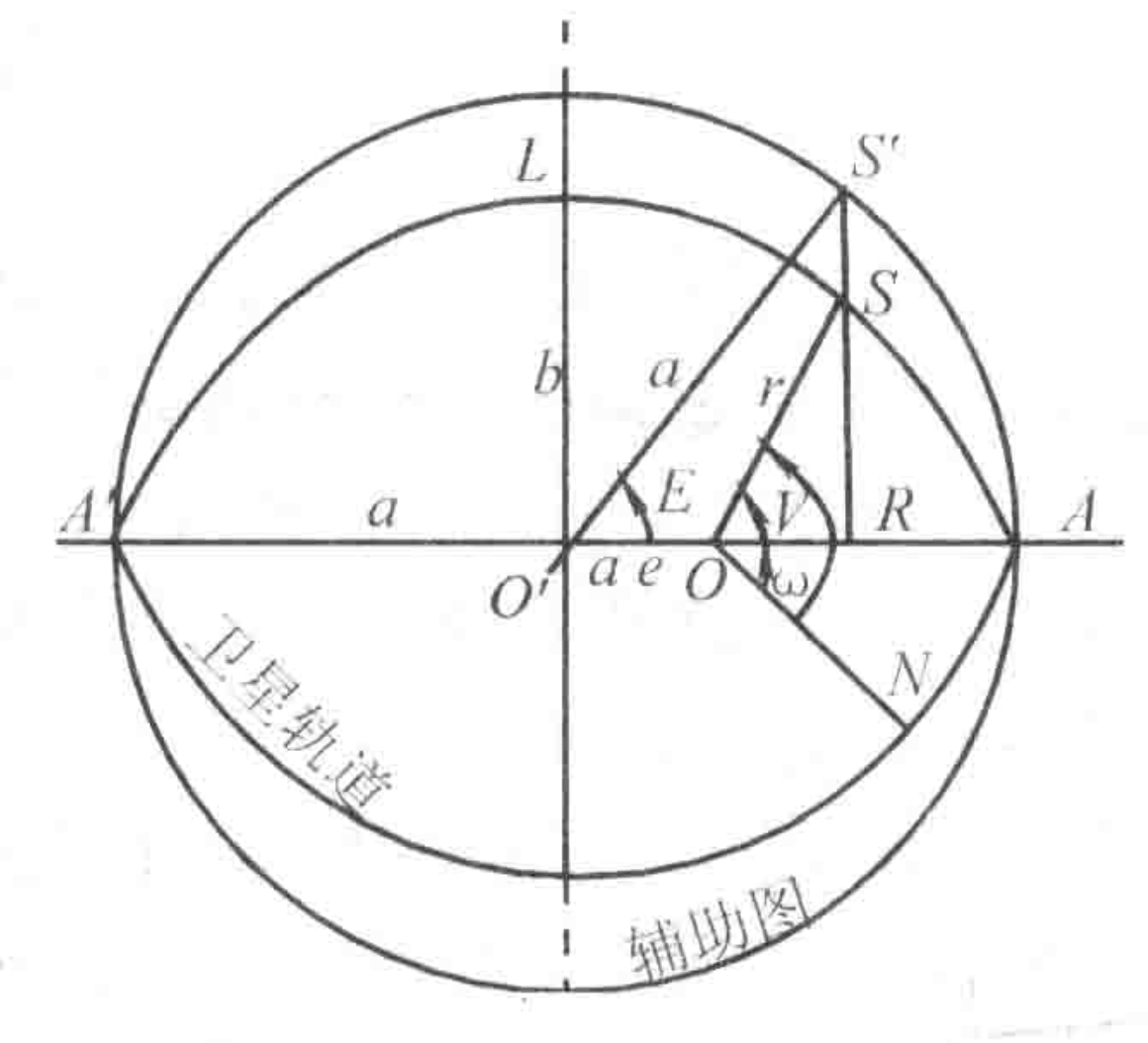
开普勒轨道参数有哪些？

由开普勒定律可知卫星运行的轨道是通过地心平面上他椭圆。开普勒轨道参数(a, e, V, Ω, i, ω)可以描述卫星的无摄运动，定义为：

a: 椭圆的长半径
e: 椭圆的偏心率
V: 卫星的真近点角(轨道平面上卫星与近地点之间的地心角距)
Ω: 升交点赤经(地球赤道平面上升交点N与春分点γ之间的地心夹角)
i: 轨道面倾角
ω: 近地点角距(轨道平面上近地点A与升交点N之间的地心角距)

其中(a, e, V)唯一确定了卫星轨道的形状、大小和卫星在轨道上的瞬时位置，(Ω, i)唯一确定了卫星轨道平面与地球体之间的相对定向，ω表达了开普勒椭圆在轨道平面上的定向。

什么是无摄运动和受摄运动？

卫星的无摄运动: 只考虑地球质心引力作用的卫星运动，将地球和卫星看做两个质点作为二体问题研究两个质点在万有引力作用下的运动。
卫星的受摄运动: 考虑了摄动力作用的卫星运动，考虑了地球引力场摄动力、日月摄动力、大气阻力、光压摄动力、潮汐摄动力对卫星运动状态的影响。在考虑摄动力的作用后，卫星的受摄运动的轨道参数不再保持为常数而是随时间变化的轨道参数。

什么是真近点角？如何计算某时刻的真近点角？

真近点角 表示从轨道距离焦点最近的点到当前为止的角度。以地球质心O为原点，x轴指向升交点N方向，自x轴按卫星运行方向旋转90^∘为y轴建立轨道平面坐标系O − xy。忽略卫星质量卫星在该平面上的运动微分方程为:

$$ \begin{cases} \mid \overset{..}{X} \mid &= - \frac{GM}{r^3} X \\ \mid \overset{..}{Y} \mid &= - \frac{GM}{r^3} Y \end{cases} $$

由微分方程同阶得到卫星运动的轨道方程:

$$ r = \frac{h^2}{GM} / \left(1 + e \cos (\theta - \omega)\right) $$

其中e、ω为新的积分常数，θ为从x轴指向卫星径向r⃗的角度。

由于 θ = ω + V且h² = GM ⋅ a(1 − e²)，因此可用真近点角V表示为:

r = a(1 − e²)/(1 + ecos V) 其中V为与时间t有关的变量，解算特定时刻的真近点角需要使用其与偏近点角和离心率之间的关系计算。

由几何关系， ∣ OR ∣ = rcos V = a(cos E − e)，即可用偏近点角E表示轨道方程为:

r = a(1 − ecos E)

整理得到:

$$ \begin{cases} \cos V &= (\cos E - e) / ( 1 - e\cos E) \\ \tan (V /2) &=\sqrt{(1 + e)/(1 - e)} \tan(E/2) \end{cases} $$

接着设卫星沿椭圆运动的周期为T，则平均角速度为:

n = 2π/T

联立开普勒第二定律和第三定律得到开普勒轨道方程为:

n(t − τ) = E − esin E 其中τ为积分常数，令M = n(t − τ)，则M岁时间t以平均角速度n变化故称M为平近点角，则:

M = nt − M₀ = E − esin E

从而成功建立t与E的数学关系从而确定t与V的数学关系。

简述GPS卫星星历的分类及其特点。

GPS 卫星星历分为预报星历和后处理星历两类:

预报星历: 又称广播星历，通常包括相对某一参考历元的开普勒轨道参数和必要的轨道摄动改正项参数。广播星历参数的选择采用了开普勒轨道参数加调和项修正的方案。 GPS 卫星的运动在二体运动的基础上加入了长期摄动和周期摄动，包括1个参考时刻，6个对应参考时刻的开普勒轨道参数和9个反映摄动力影响共计16个参数。参数定义如下:
t_oe :星历表参考历元
M₀ :按参考历元t_oe计算的平近点角
e :轨道偏心率
$\sqrt{a}$ :轨道长半径的平方根
Ω₀ :按参考历元t_oe计算的升交点赤经
i₀ :按参考历元t_oe计算的轨道倾角
ω :近地点角距
$\overset{.}{\Omega}$ :升交点赤经变化率
$\overset{.}{I}$ :轨道倾角变化率
Δn :由精密星历计算得到的卫星平均角速度与按给定参数计算所得的平均角速度之差
C_uc/C_us :纬度幅角的余弦/正弦调和项改正的振幅
C_rc/C_rs :轨道半径的余弦/正弦调和项改正的振幅
C_ic/C_is :轨道倾角的余弦/正弦调和项改正的振幅

其中Δn中包括了轨道参数ω的长期摄动。此外还包括一些数据质量和卫星健康参数:

IODE(AODE) :星历表数据龄期，用于版本控制和数据有效性
IODC :星钟的数据龄期
a₀, a₁, a₂ :分别表示卫星钟差，卫星钟速和卫星钟速变率
卫星精度和卫星健康
GPD :周数
T_gd :载波L₁、L₂的电离层时延误差
后处理星历: 是一些国家某些部门根据各自建立的卫星跟踪站所获得的对 GPS 卫星的精密观测资料，应用与确定广播星历相似的方法而计算的卫星星历。它可以向用户提供在用户观测时间内的卫星星历避免了星历外推的误差。后处理星历文件记录中每隔 15 分钟给出目前在轨卫星的三维坐标信息和卫星钟差甚至卫星的三维速度及相关精度指标信息。

如何计算 GPS 卫星在协议地球坐标系下的坐标？

计算 GPS 卫星在协议地球坐标系下的坐标分为以下步骤:

计算卫星运行的平均角速度n

根据开普勒第三定律卫星运行的平均角速度n₀计算方式为:

$$ n_0 = \sqrt{GM / a^3} = \sqrt{\mu} / (\sqrt{a})^3 $$ 其中μ为WGS-84坐标系中的地球引力常数。则卫星运行平均角速度n = n₀ + Δn，Δn为卫星电文给出的摄动改正数。

计算归化时间t_k

改正观测时刻t = t′ − Δt由对观测时刻t′改正得到，其中:

$$ t = a_0 + a_1(t’ - t_{oe}) + a_2(t’ - t_{oe})^2

然后将改正观测时刻t归化到 GPST 得到:

$$ t_k = t - t_{oe}

其中t_k为相对于参考时刻t_oe的归化时间。

计算真近点角V_k

根据参考时刻t_oe得到M₀计算观测时刻卫星平近点角M_k:

M_k = M₀ + nt_k

根据得到此时偏近点角E_k的表达式为:

E_k = M_k + esin E_k

使用迭代法求解E_k从而根据进一步得到真近点角V_k。

计算经过摄动改正的轨道参数

根据得到的真近点角V_k和卫星星历得到的ω由几何关系得到:

Φ_k = V_k + ω

根据卫星星历获得的六个轨道参数余弦/正弦摄动改正项得到摄动改正项:

$$ \begin{cases} \delta u &= C_{uc} \cdot \cos (2 \Phi_k) + C_{us} \cdot \sin (2\Phi_k) \\ \delta r &= C_{rc} \cdot \cos (2 \Phi_k) + C_{rs} \cdot \sin (2\Phi_k) \\ \delta i &= C_{ic} \cdot \cos (2 \Phi_k) + C_{is} \cdot \sin (2\Phi_k) \\ \end{cases} $$ 其中δu、δr、δi分别为升交距角u、卫星矢距r⃗和轨道倾角i的摄动量，则经摄动改正计算后三个参数为:

$$ \begin{cases} u_k &= \Phi_k + \delta u \\ r_k &= a(1 - e \cos E_k) + \delta r\\ i_k &= i_0 + \delta i + \overset{.}{I} \cdot t_k \end{cases} $$

计算卫星在轨道平面坐标系的坐标

卫星在定义的轨道平面坐标系坐标为:

$$ \begin{cases} x_k &= r_k \cos u_k \\ y_k &= r_k \sin u_k \end{cases} $$

计算观测时升交点经度Ω_k

观测时刻升交点赤经由参考时刻t_oe的升交点赤经Ω_oe和卫星星历得到的升交点赤经变化率$\overset{.}{\Omega}$计算:

$$ = _{oe} + t_k

从而升交点经度Ω_k可由Ω与春分点和格林尼治子午线之间的角距视恒星时GAST得到:

$$ _k = -

其中GAST根据每周的起始时刻位置GAST_w和地球自转速度ω_e得到:

$$ = _w + _e t

$$ 其中t为观测时刻相对于一周开始经过的时间。联立,,和得到:

$$ \Omega_k = \Omega_0 + (\overset{.}{\Omega - \omega_e})\cdot t_k - \omega_e \cdot t_{oe} $$

计算卫星在协议地球坐标系中的直角坐标

将卫星在轨道平面直角坐标系中的坐标进行旋转变换可得卫星在地固坐标系中的三维坐标:

$$ \begin{pmatrix} X_k \\ Y_k \\ Z_k \end{pmatrix} = \begin{pmatrix} x_k \cos \Omega_k - y_k \cos i_k \sin \Omega_k \\ x_k \cos \Omega_k + y_k \cos i_k \cos \Omega_k \\ y_k \sin i_k \end{pmatrix} $$

进一步考虑极移影响得到卫星在协议地球坐标系中的坐标:

$$ \begin{pmatrix} X \\ Y \\ Z \end{pmatrix}_{\text{CTS}} = \begin{pmatrix} 1 & 0 & X_p \\ 1 & 1 & -Y_p \\ -X_p & Y_p & 1 \\ \end{pmatrix} \begin{pmatrix} X_k \\ Y_k \\ Z_k \end{pmatrix} $$

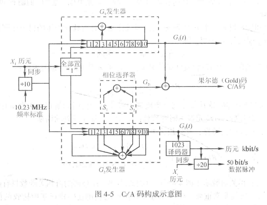
简述GPS信号的分类。

GPS信号包含载波、测距码和数据码，使用f₀ = 10.23MHz作为基本频率发生。测距码和数据码通过调相技术调制到载波上。

载波: 使用 L 波段的两种载波：(1)f_L₁ = 154 × f₀ (2)f_L₂ = 120 × f₀
测距码: 分为粗码(C/A码)和精码(P码)两种
数据码: 按照特定格式进行播报

什么是PRN？简述其产生原理。

伪随机噪声码(PRN)是一个具有一定周期的取值为0和1的离散符号串。具有高斯噪声良好的自相关特征和确定的编码规则。GPS 技术采用 m 序列产生PRN。对于一个k级反馈移位寄存器，产生步骤为:

设定初始时刻状态 PRN₀ = (a₀⁰, a₁⁰, …, a_k − 1⁰)
设定用于产生信号的位置序列 L = (l₁, l₂, …, l_n), (0 ≤ l₁ < l₂ < … < l_n ≤ k − 1)
对于任意时刻t(t ≥ 0)信号，根据PRN_t = (a₀^t, a₁^t, …, a_k − 1^t)位置序列L上的信号模2相加得到新信号$A=(\sum_{i=1}^n a_{l_i}) \mod{2}$
则t + 1时刻信号为PRN_t + 1 = (a₁^t, a₂^t, …, A)
递推执行上述过程，生成周期为2^k − 1的随机码序列

什么是导航电文？试述其格式和内容。

导航电文是用户用来定位和导航的数据基础，主要包括卫星星历、时钟改正、电离层时延改正、工作状态信息以及C/A码转换到捕获P码的信息。

卫星电文的基本单位是长1500bit的一个主帧需要30秒进行传输。一个主帧包含5个子帧，其中第1,2,3子帧各有10个字码，每个字码30bit；第4,5子帧各有25个页面共37500bit。其中第1,2,3子帧每30秒重复一次，内容每半小时更新一次；第4,5子帧750秒播完一次后进行重复，内容在注入新的导航数据后才会更新。一个主帧包含以下信息:

遥测码(TLW) 位于各子帧的开头用来表明卫星注入数据的状态。
转换码(HOW) 位于每个子帧的第2个字码用来帮助用户从捕获的C/A码转换到捕获P码的Z计数。
第一数据块位于第1子帧的3-10字码，主要包括标识码和一些时间和质量控制信息。
第二数据块位于第2和第3子帧，内容表示 GPS 卫星的星历。
第三数据块位于第4和第5两个子帧，内容包括了所有 GPS 卫星的历书数据。

简述GPS测量主要误差的分类。

按照误差来源分为以下四种类型:

卫星部分: (1)星历误差;(2)卫星钟差;(3)相对论效应
信号传播: (1)电离层误差;(2)对流层误差;(3)多路径效应
信号接收: (1)接收机钟差;(2)位置误差;(3)天线相位中心变化
其他影响: (1)地球潮汐;(2)负荷潮

简述GPS测量各类误差的影响特性。

系统误差是GPS测量的主要误差源，包括卫星的星历误差、卫星钟差、接收机钟差以及大气折射的误差等。以下分类简述其影响特性。

与卫星有关的误差

星历误差在一个观测时间段内属于系统误差特性，是一种起算数据误差，将严重影响单点定位的精度。
卫星钟差包括钟差、频偏、频漂等产生的误差，也包括钟的随机误差。卫星钟的偏差一般可表示为的二阶多项式形式，参数a₀, a₁, a₂由卫星的地面控制系统根据前一段时间的跟踪资料和GPS标准时推算出来再通过导航电文提供给用户。
相对论效应主要取决于卫星的运动速度和重力位，会改变卫星钟的频率。

与信号传播有关的误差

电离层折射发生在 GPS 信号通过电离层时信号的路径会发生弯曲并改变传播速度。电磁波在这种介质内传播时速度与频率有关。
对流层折射与地面气候、大气压力、温度和湿度变化密切相关，对流层折射的影响与信号的高度角有关，一般采用改正模型进行削弱。
多路径误差发生在测站周围的反射物所反射的卫星信号进入接收机天线，将和来自卫星的信号产生干涉，从而使观测值偏离真值。

与接收机有关的误差

接收机钟差为接收机钟与卫星钟间的同步差，通过在卫星间求一次差来消除接收机的钟差。
接收机位置误差包括接收机天线相位中心相对测站标石中心位置的误差。
天线相位中心位置的偏差和GPS天线相位中心与GPS天线设计、制造工艺及材料有关，也与观测环境、时间、季节及气象条件等多种因素有关。

如何消除多路径误差影响？

削弱多路径误差主要有三点:

选择合适的站址: (1)应远离大面积平静的水面；(2)测站不宜选择在山坡、山谷和盆地中；(3)离开高层建筑物
设置合适的天线特性: (1)在天线中设置抑径板; (2) 对极化特性不同的反射信号应该有较强的抑制作用

从产生原理看，反射波和直接波间的相位延迟θ为:

$$ \theta = \Delta \cdot \frac{2\pi}{\lambda} = 4 \pi H \sin (\frac{z}{\lambda}) $$ 其中λ为载波的波长。从而由于反射波一部分能量被反射面吸收，GPS接收天线为右旋圆极化结构也抑制反射波的功能。

试写出测码伪距观测方程，说明各参数意义并解释为何需观测至少4颗卫星才可实现定位？

测码伪距观测方程的基本形式为:

P = ρ + c ⋅ δt + ϵ

其中P为伪距测量值，ρ为实际几何距离δt为卫星钟差，ϵ为观测误差项。

整理上式，对于任一卫星而言:

$$ \begin{cases} P_r^s &= c(T_r - T^s) \\ T_r &= t_r + \delta t_r \\ T^s &= t^s + \delta t_s \\ \end{cases} $$ 其中 T 为观测时刻，t 为真时刻，联立化简得到:

$$ \begin{aligned} P_r^s &= c(t_r - t^s ) + c(\delta t_r - \delta t^s) =\rho_r^s + c(\delta t_r - \delta t^s) \\ &= \sqrt{(x_r - X^s)^2 + (y_r - Y^s)^2 + (z_r - Z^s)^2} + c(\delta t_r - \delta t^s) \end{aligned} $$ 其中 ρ 为用户与卫星之间的伪距， δt_r 为用户误差，δt_s 为接收的卫星误差。其中(X^s, Y^s, Z^s, δ^s)为卫星上的未知量，因此需要联立四个卫星观测方程:

留下未知量为(x_r, y_r, z_r, δt_r)分别表示用户的三维空间坐标和接收机钟差。

试写出载波相位观测方程，在卫星数为K颗的前提下，在某测站上需观测至少几个历元才可实现未知数的解算？

载波相位观测方程为:

Φ = ρ + δτ + ϵ + N 其中Φ为接收到的载波相位观测值，ρ为卫星与接收机之间的真实几何距离，δτ为钟差改正项，ϵ为观测误差项，N为整数倍波长(整周模糊度)。

对于定点测量，同步观测数和观测历元数需要满足关系:

n_sn_t ≥ 3 + n_t 其中n_s为同步观测数即卫星数，n_t为观测历元数，因此在题设条件下需要的历元数为:

$$ n_t \geq \frac{3}{k-1} \quad (k \geq 2) $$

试述观测量线性组合的几种形式、特点。

单频观测量组合是对于单频的观测量将伪距测量和载波相位观测量进行组合。由于其仅依赖一个频率的观测，易受大气延迟和多路径效应影响，抗干扰能力弱且精度较低。将伪距观测和载波相位观测组合可以进行整周模糊度解算。
双频观测量组合是通过组合两个不同频率（如L1和L2）的观测量组合。双频组合可以有效消除电离层延迟对测量的影响，通过整合不同频率的信息，**定位精度显著提高}。
差分观测组合是利用基准站和移动站的观测量进行差分计算。通过差分计算，可以消除共同误差并进行实时修正
加权线性组合是对不同观测量施加权重进行组合，通常用于处理不同精度和信噪比的观测量。可以根据观测质量动态调整权重，提高定位精度。灵活性高并可以有效抑制低质量观测对最终解的影响

试述单差、双差、三差的含义、作用。

GPS 载波相位观测值可以在卫星间求差，在接收机间求差，也可以在不同历元之间求差。各种求差法都是观测值的线性组合。设测站1和测站2分别在t_i时刻和t_i + 1时刻对卫星k和卫星j进行载波相位观测，观测值分别为Φ₁^k(t_i),Φ₂^k(t_i),Φ₁^k(t_i + 1),Φ₂^k(t_i + 1)和Φ₁^j(t_i),Φ₂^j(t_i),Φ₁^j(t_i + 1),Φ₂^j(t_i + 1)

单差指将观测值直接相减的过程，常用单差是在接收机间求一次差，得到虚拟观测值SD₁₂^k(t) = Φ₂^k(t_i) − Φ₁^k(t_i) 和 SD₁₂^j(t) = Φ₁²j(t_i) − Φ₁^j(t_i)从而可以消除卫星钟差的影响。
双差指对单差观测值继续求差，常用双差是在接收机之间求单差后再在卫星间求双差(星站二次差分)，得到虚拟观测值DD₁₂^kj(t_i) = SD₁₂^j(t) − SD₁₂^k(t) = Φ₂^j(t_i) − Φ₁^j(t_i) − Φ₂^k(t_i) + Φ₁^k(t_i)，在多次同步观测组成法方程后可以解算出待定点坐标改正数、钟差等未知参数。
三差指对双差观测值继续求差，常用三差在接收机、卫星和历元之间求三次差，得到虚拟观测值TD₁₂^kj(t_i, t_i + 1) = DD₁₂^kj(t_i + 1) − DD₁₂^kj(t_i)，可以消除与卫星和接收机有关的初始整周模糊度项N₀等。

简述CORS的分类。

CORS系统是参考站系统(Continuous Operation Reference System)的简称，是局地固定 GPS 基准站组成的网络系统，专门接收 GPS 信号的称 GPS CORS，但目前测站都转向多卫星源的 GNSS CORS，按照服务方式可分为:

实时CORS: 提供实时差分定位服务，用户可以即时获取高精度的位置信息。主要用于动态应用，如车辆定位、无人机导航等。
静态CORS: 提供后处理服务，用户需下载数据后进行离线处理。适用于高精度测量和地形测绘等静态应用。